I’ve been thinking about machine learning training order on and off for a little while now. Sometimes these thoughts bubble up while playing Switch. Sometimes it’s while pulling into the parking lot of some big-box store, but I digress.

Let’s consider some sort of supervised learning system (like the Not Hotdog image classifier from Silicon Valley). As best as I remember I was always taught to feed in training data in random order. This strategy sounds reasonable enough, but is random order actually the best strategy or is it simply an easy strategy? Or maybe training order doesn’t matter much at all?

Eventually I flipped the logic on its head and asked myself why we don’t simply teach kids material in random order at school? If random training order was so great or if it didn’t matter at all shouldn’t something like this work fine? Yeah, yeah, there’s a huge difference between a dinky neural net and a developing child, but this analogy was so annoyingly simple it stuck like a thorn in my side. After a couple more sessions of pondering I got the question narrowed down enough to the point where I could start creating an experiment around it.

Question, Hypothesis

Q — To what extent does training order affect image classifier performance?

H — It certainly seems like it should matter, doesn’t it? Maybe there’s even a scheme that can beat random training order…

Experiment Design

The Foundation

When I mentioned dinky neural net I wasn’t joking. I didn’t want to burn weeks of cloud credits, so I decided to base everything on PyTorch’s CIFAR-10 image classifier tutorial. The data set and CNN architecture were simple enough that everything could run on my laptop without trouble.

NOTE: CIFAR-10 is an older and much, much smaller benchmark data set than something contemporary like ImageNet, but it’s still useful for learning and small prototypes. The training set is composed of 50,000 images evenly spread across 10 image classes.

The Scheme

Now to the meat of the experiment: how would I order the training data? In fuzzy terms I wanted to sort the images by how much “good stuff” was in each one. Reaching way back into the grad school brain, I settled on using the entropy of the raw pixel values converted to grayscale. Visually, homogenous images have low entropy, and chaotically textured images have high entropy. It was far from a perfect metric, but in keeping with my “small data” theme it seemed like a good place to start.

The Tests

As I was playing around with sloppy initial code, the loss and accuracy numbers with entropy sort were getting interesting. After some pondering I settled on the following setups to test.

• Random Order (control case)
• Global Entropy Sort, Ascending
• Global Entropy Sort, Descending
• Grouped Entropy Sort within Image Class, Ascending
• Grouped Entropy Sort within Image Class, Descending

Each of the above configurations were tested with various training set sizes based on the original CIFAR-10 training sets (100%, 90%, 80%, 70%, 60%, 50%, 40%, 30%, 20%, 10%). Smaller training sets were generated by taking the 100% sized training set and dropping images from the end of the list, so in entropy sort configurations this forcibly removed either high or low entropy training images. In the random order configuration it simply starved the net of training data.

Grouped entropy sort was included to make the sorting more fair because average entropy was not equivalent across image classes. In this mode training images were sorted by entropy within their respective image classes, and the final ordering would draw from each sorted image class in a round-robin fashion.

Results: Random Order

The key random ordered test was when training set size was set to 100%. This configuration made the test essentially the same as the original PyTorch tutorial. Naturally, I expected to see very similar results.

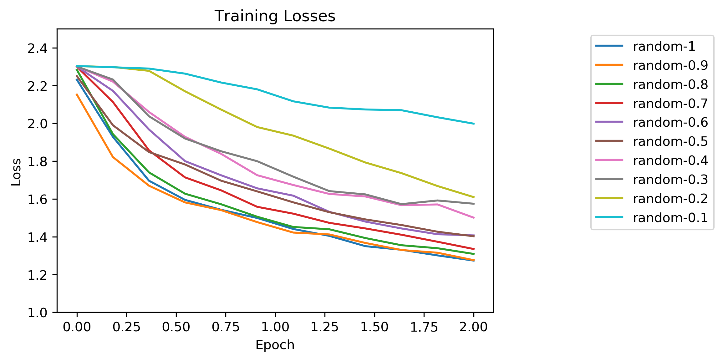
This is a standard chart plotting loss versus normalized training epoch, where the number of iterations per epoch is equal to the training set size. The results looked pretty textbook with loss leveling out asymptotically. As one would expect, the tests with smaller training sets produced shallower loss curves, indicating that the optimization had difficulty converging.

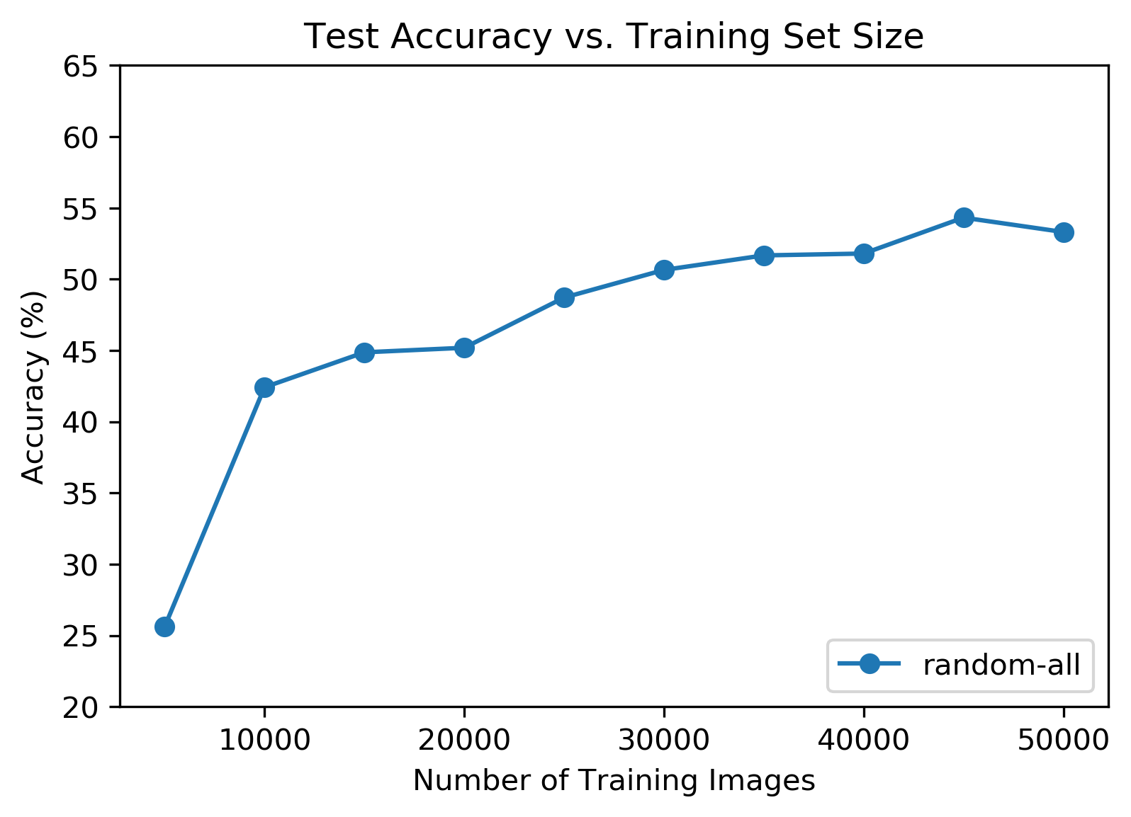
This chart shows total accuracy across all image classes against training set size. Again, these results seemed intuitive, where accuracy decreased with training set size. Accuracy achieved on the full training set was 53%, which was consistent with the number achieved in the original PyTorch tutorial.

Results: Global Entropy Sort Ascending

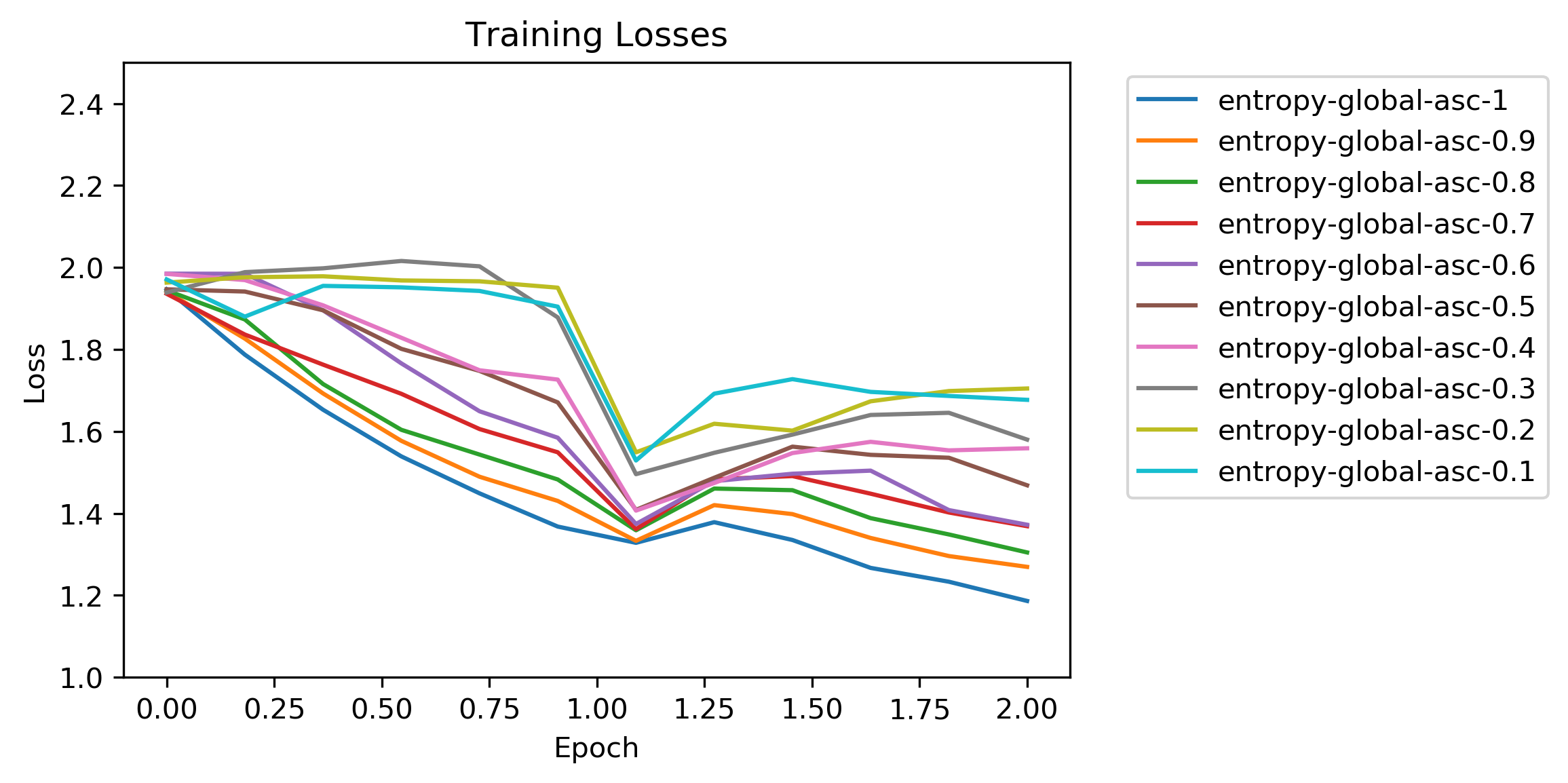
The shape of these loss curves was more erratic than the random ordered tests. The interesting thing here was the upwards loss bump at the start of the second epoch. This was when the optimization finished the high entropy images at the end of the first epoch and switched to low entropy images again.

It’s also worth pointing out that the loss started at a noticeably lower value than the random ordered tests. Maybe there was less difference image-to-images because of the entropy sorting, and this helped the optimization?

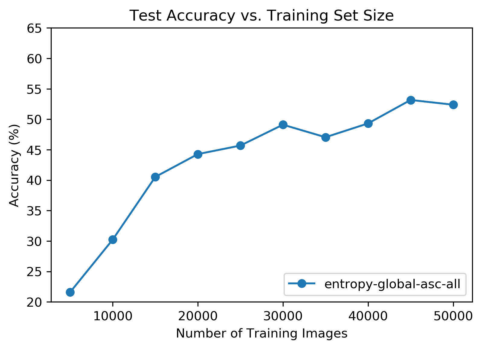
No surprises here. Accuracy took a dive as the training set size shrank. Even though the loss chart looked very different from the random ordered tests, peak total accuracy was roughly the same.

Results: Global Entropy Sort Descending

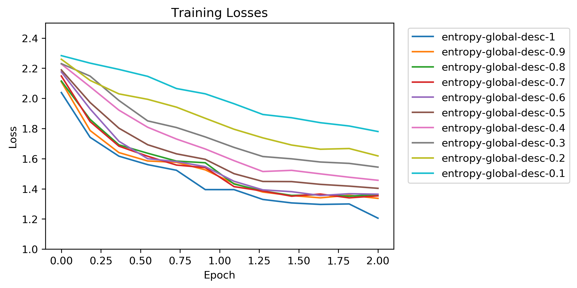
This loss chart was more normal looking than the version from the previous section’s test parameters. For large training set sizes the initial loss did still start at a lower value than the randomly ordered tests.

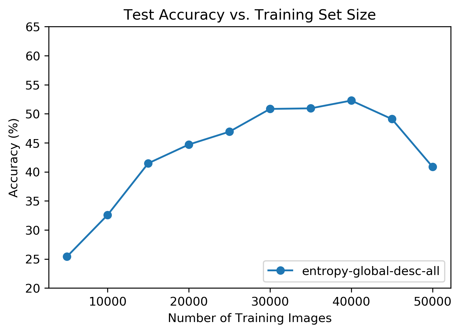
This was the most interesting chart so far! The largest training set size performed relatively poorly, and peak accuracy occurred at 40,000 training images (80%). It’s worth pointing out that in this configuration 10,000 low entropy images were kept out of the training set. Something about these images reduced total accuracy.

Results: Grouped Entropy Sort Ascending

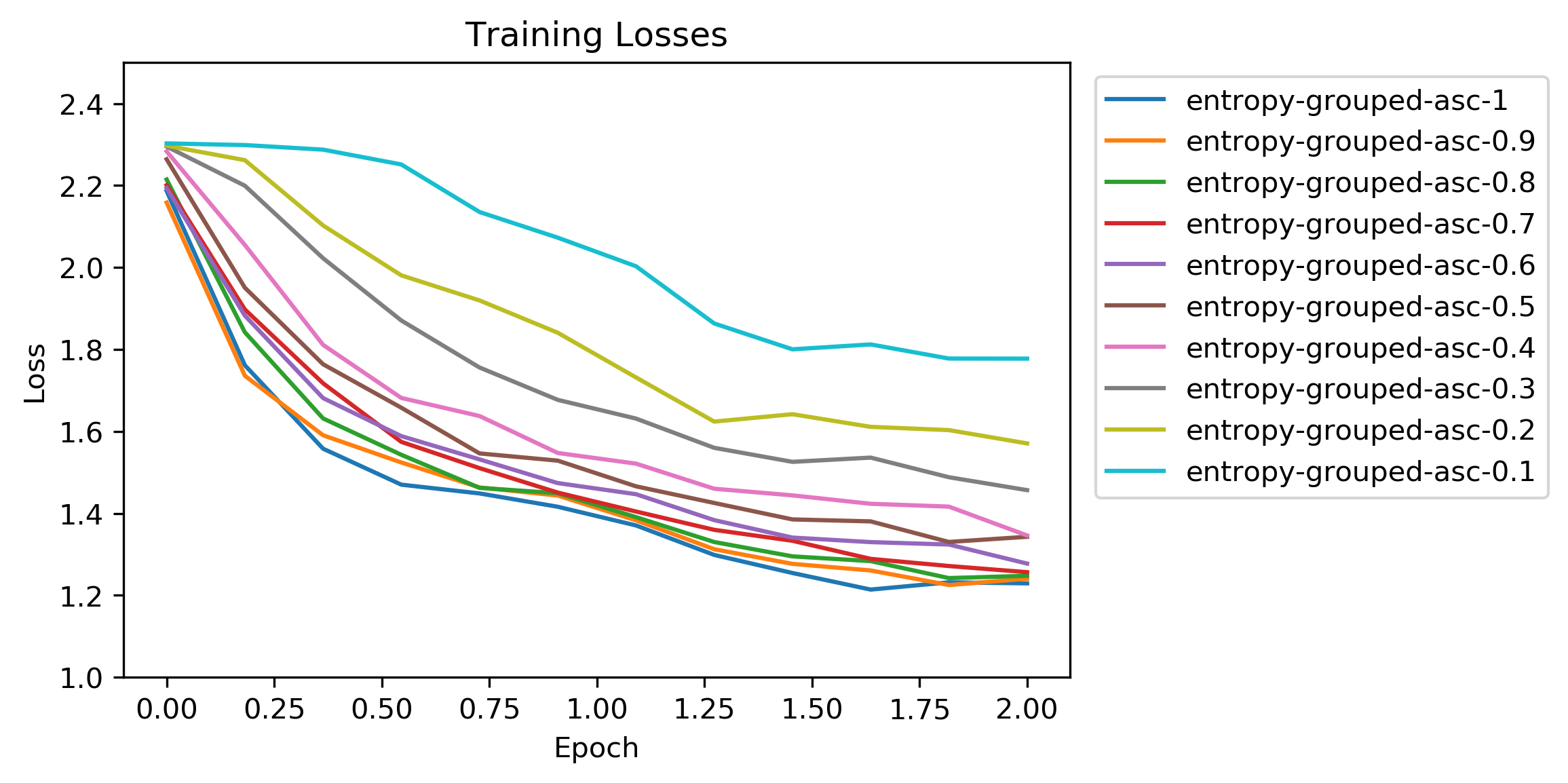
Unlike the ascending global entropy sort tests this loss chart did not have the weird dip and hump between epochs. The lower initial loss values from that test were also not present here. This chart looked pretty similar to the random ordered tests.

It’s possible that the lower initial loss in the global entropy sort tests was from some image classes having inherently higher or lower entropies, which would result in runs of training data that were not distributed uniformly across image classes. This possible unfairness in entropy distribution was the original reason for including the grouped entropy sort tests.

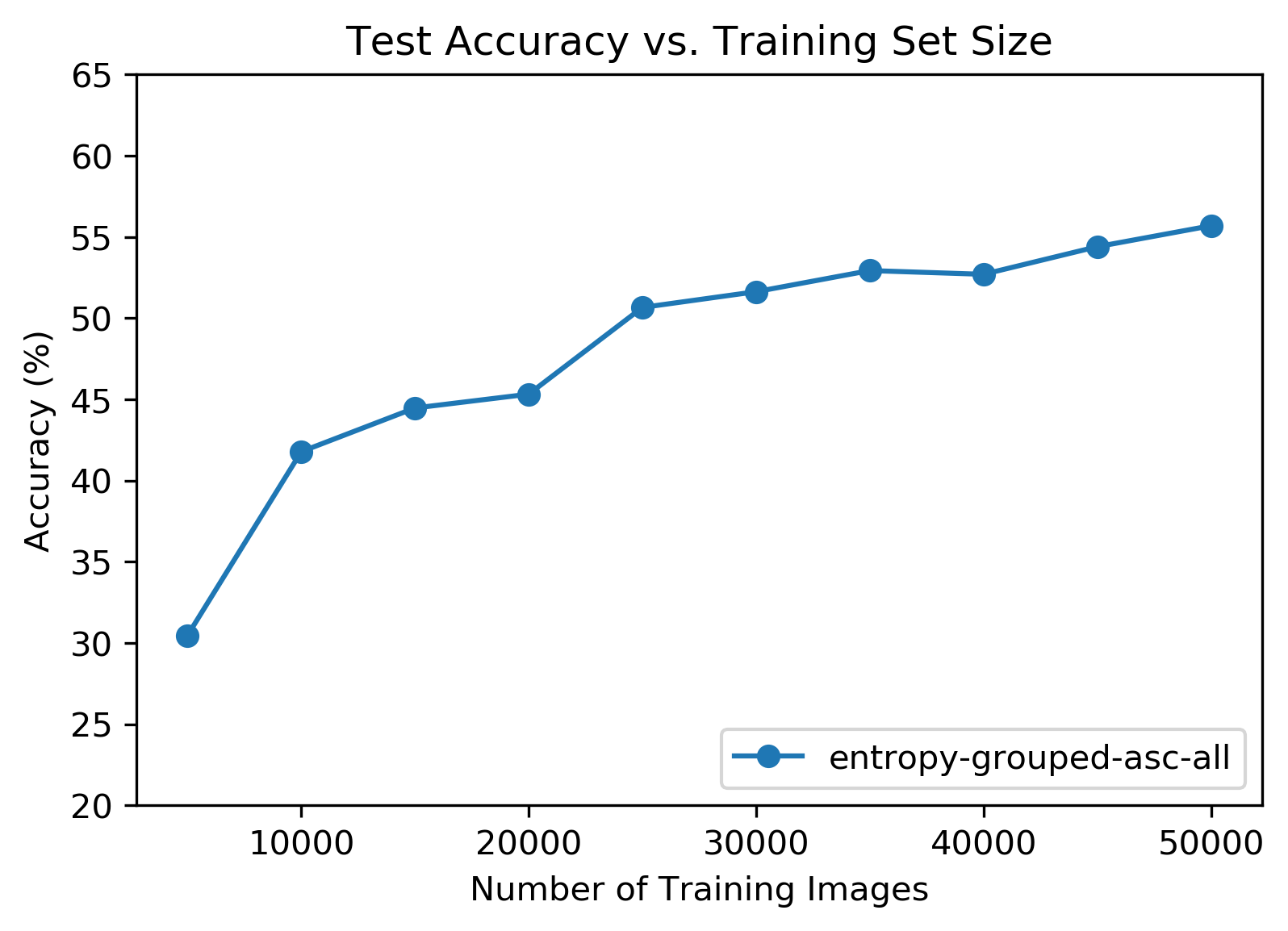
Accuracy results looked pretty normal yet again. Peak total accuracy was roughly the same, too.

Results: Grouped Entropy Sort Descending

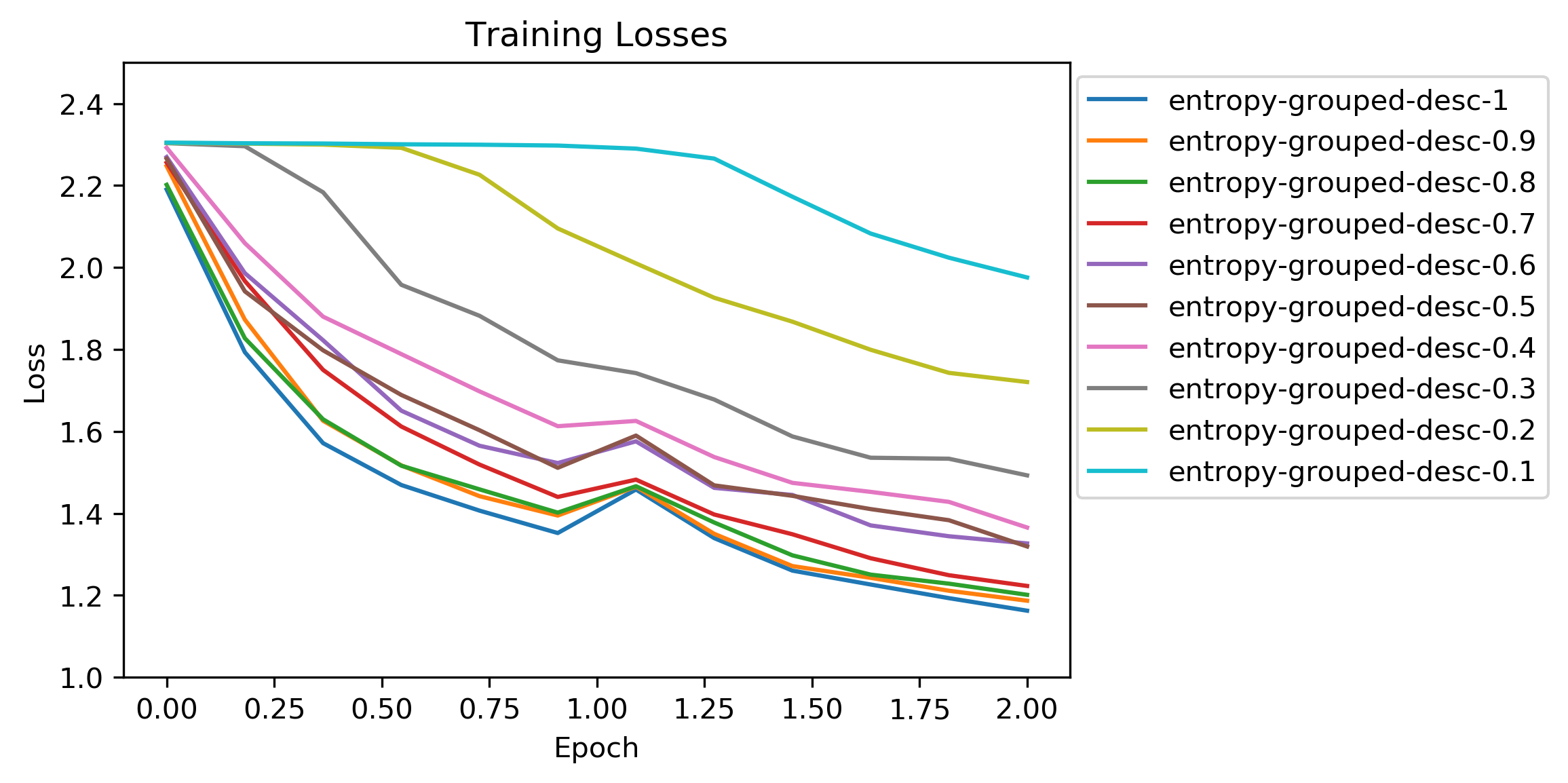
That weird bump came back but this time on the descending tests! I didn’t have an explanation for it. Again, the initial loss started at around the same value as the random ordered tests.

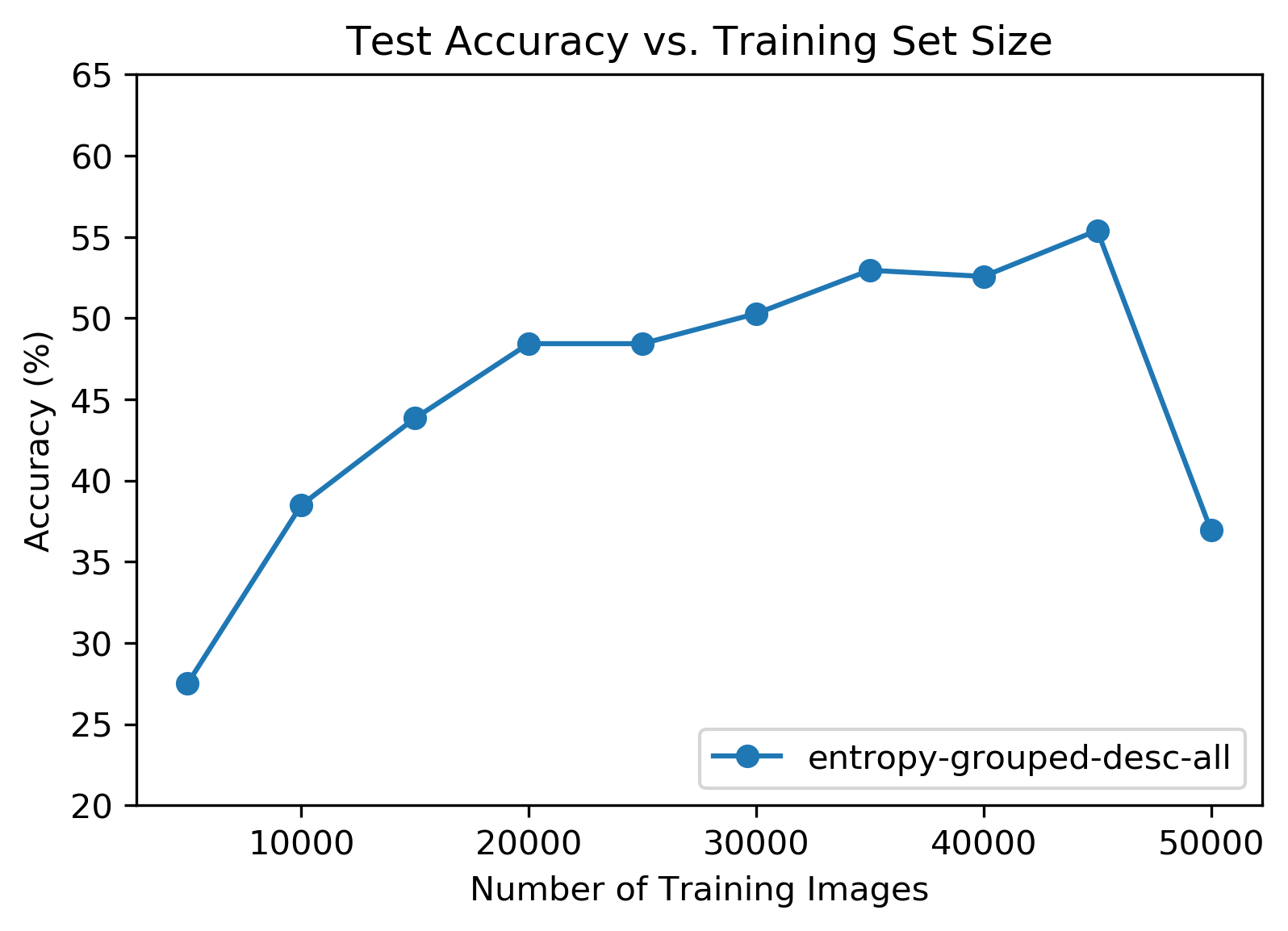
The fun accuracy curve was also back and very pronounced this time! Unlike the mysterious loss behavior, this accuracy curve consistently showed up on both sets of descending order tests. This lends more credence to the theory that some of the low entropy training images were not helping.

Conclusion

Answer the Damn Question

Test Type	Test Accuracy (Full Training Set)
Random Order	53%
Global Entropy Sort Ascending	52%
Global Entropy Sort Descending	40%
Grouped Entropy Sort Ascending	55%
Grouped Entropy Sort Descending	36%

So does training order affect classifier performance? It does! Unfortunately the effect shown above is of the performance decreasing variety, but that’s still an effect as it relates back to the original question.

Takeaways

The accuracy curves of the descending entropy sort tests (both global and grouped) were the most interesting part of the experiment. They suggest that some of the low entropy training images in the CIFAR-10 set might be irrelevant or even harmful to classifier performance.

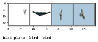
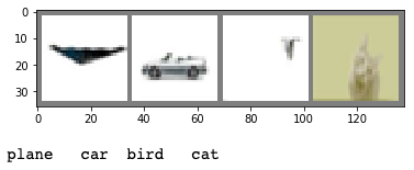
Above are the 4 lowest entropy images from the global entropy sort (top) and grouped entropy sort (bottom) configurations. The obvious thing here is that these images have either had their backgrounds removed or have naturally homogenous backgrounds.

Mysteriously, these hypothetical “dud” training images did not appear to lower accuracy when either random training order or ascending sort order was used. The accuracy hit only occurred in descending sort order tests where the low entropy images came at the end of the training loop. Is there such a thing as ending training on a bad note?

The other interesting part is that accuracy on the descending sort order tests became competitive with random order once enough of the low entropy images were omitted from the training set even though the size of the training set was smaller. Perhaps there is a way to heuristically prune training data without significantly harming performance. Such a method would save time and money, and maybe it would even be useful for transfer and federated learning.

Code

Last but absolutely not least, the code for this experiment is available here. The above plots and corresponding trained models are included in the repository.